01 The question
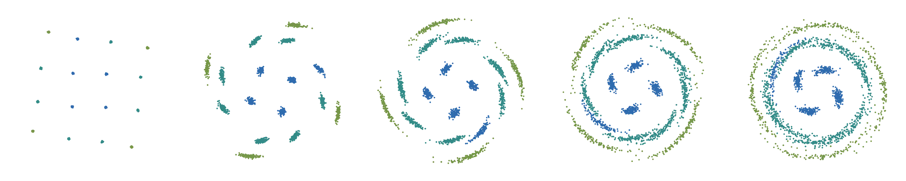
Long fibre links carry data as light whose amplitude and phase both encode bits. Push more power into the fibre and the signal gets cleaner, until the glass itself starts to bend the light: the brighter a symbol, the more its phase turns. Amplifier noise makes that turn random. This nonlinear phase noise is the wall that limits how far a link can reach.
The usual fix needs a model of the fibre. The thesis asks whether a receiver can learn its decisions from the received symbols alone, with support vector machines and random forests, and no knowledge of the link.
02 Light as a carrier
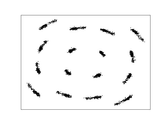
A coherent transmitter writes each symbol as one point in the plane of amplitude and phase, the constellation. More points carry more bits per symbol, but they sit closer together, so less noise is enough to push a symbol across into its neighbour's territory.
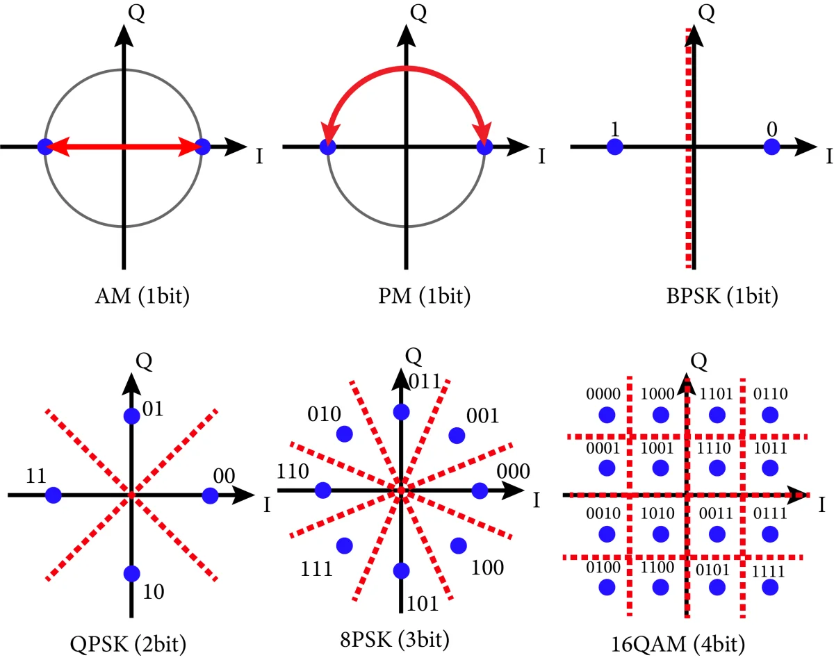
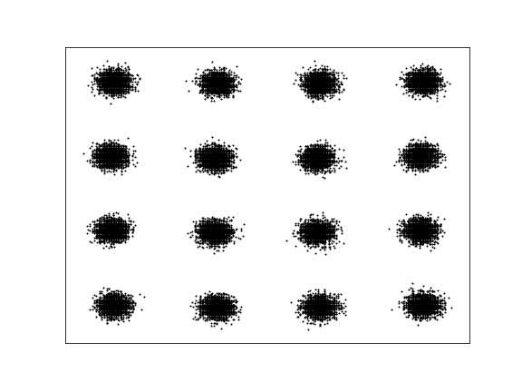
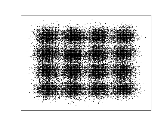
Ordinary noise blurs every point the same way, in every direction. A receiver handles it with straight decision lines halfway between the points.
 (full size, opens in a new tab)
 (full size, opens in a new tab)
 (full size, opens in a new tab)
03 When the glass bends the light
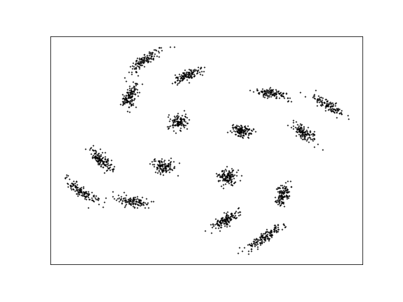
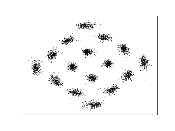
At high power the fibre's refractive index depends on the light's own intensity: the Kerr effect. Each symbol picks up a phase turn proportional to its power, so the outer points of a constellation turn further than the inner ones. Noise added by every amplifier changes the power a little, and the Kerr effect turns that into random phase. This is the Gordon–Mollenauer effect, and the constellation becomes a spiral that straight lines cannot separate.
 (full size, opens in a new tab)
 (full size, opens in a new tab)
Try it below. Pick a format, add distance, raise the power. Too little power and amplifier noise wins; too much and the spiral wins. Then switch the receiver to learned regions.
- Bits per symbol
- 4
- Wrong, nearest
- 291 / 1024
- Wrong, learned
- 14 / 1024
- Spiral
- 1.03 rad
+ sent● received● decided wrongShading: decision regions
Three things to notice in the model. QPSK barely suffers: all its points share one ring, so they turn together and the receiver takes the turn out. 64-QAM carries three times the bits and breaks first. 16-APSK puts its 16 points on two rings, which holds up better than the square grid under the same noise.
04 Learning the decision
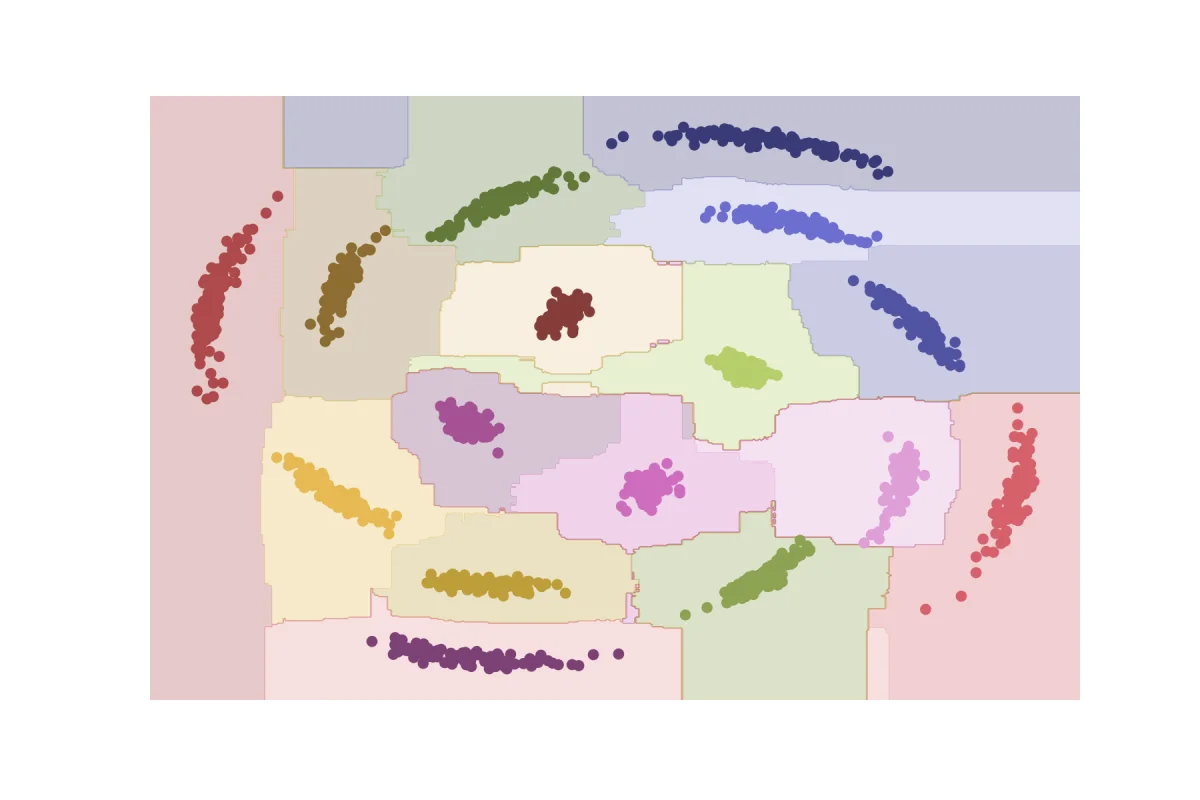
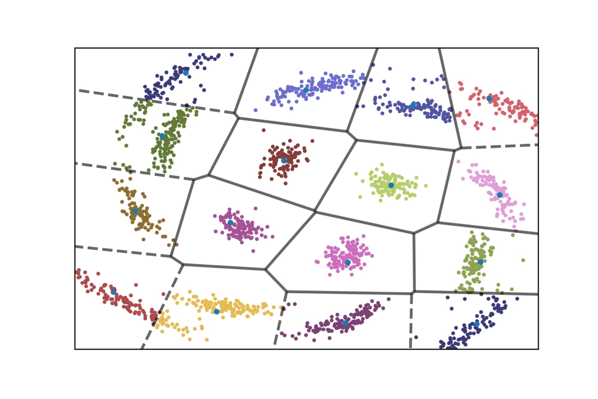
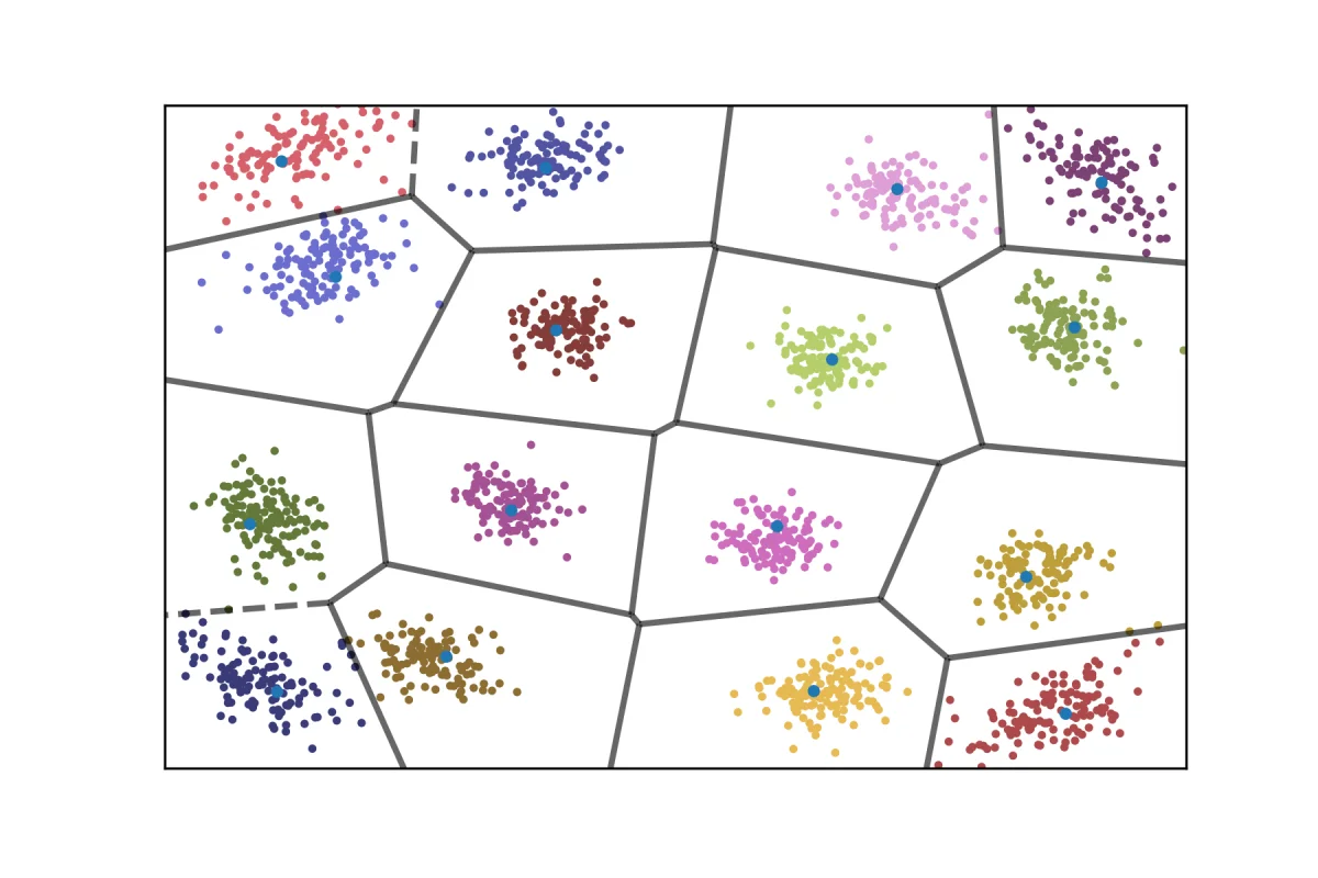
Instead of modelling the fibre, the thesis trains a classifier on received symbols whose values are known, then lets it draw the decision regions. The regions bend to follow the spiral. Two classifiers learn the same data differently: the random forest cuts the plane into boxes, the support vector machine draws smooth curves.
 (full size, opens in a new tab)
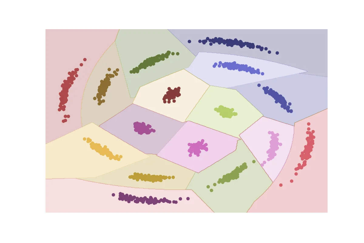 (full size, opens in a new tab)
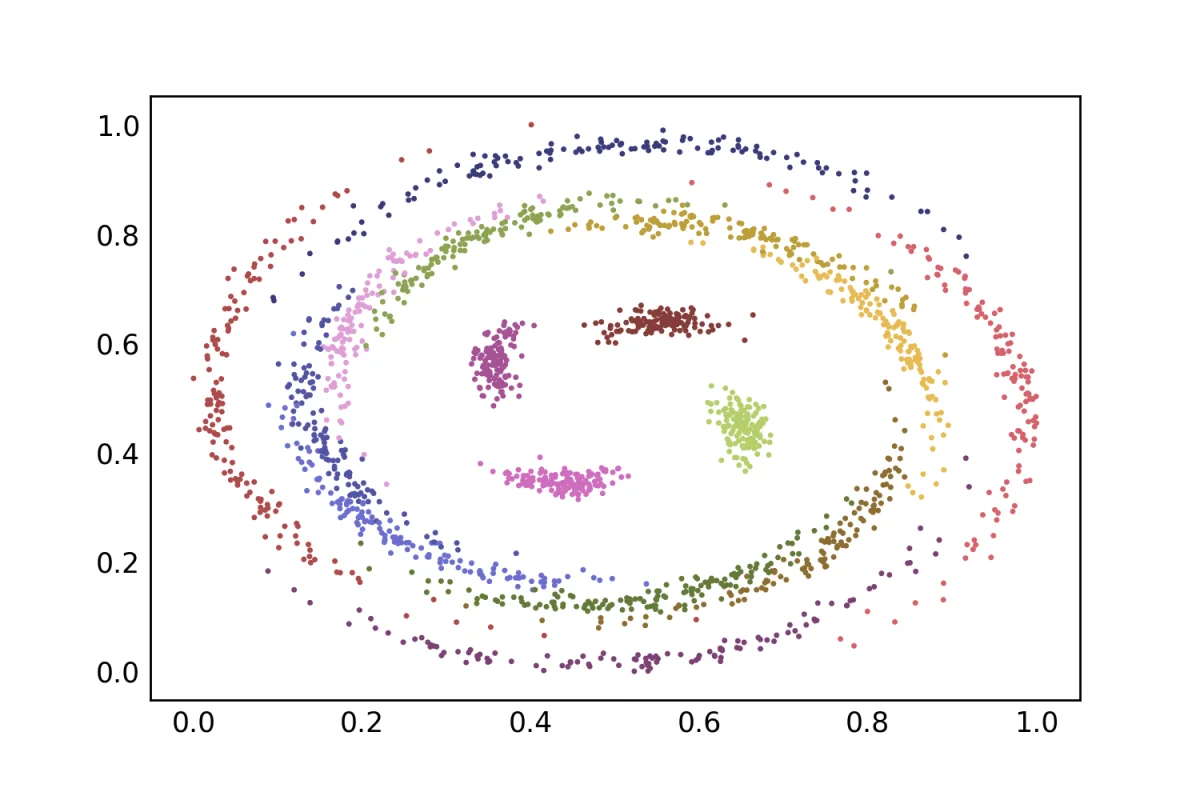 (full size, opens in a new tab)
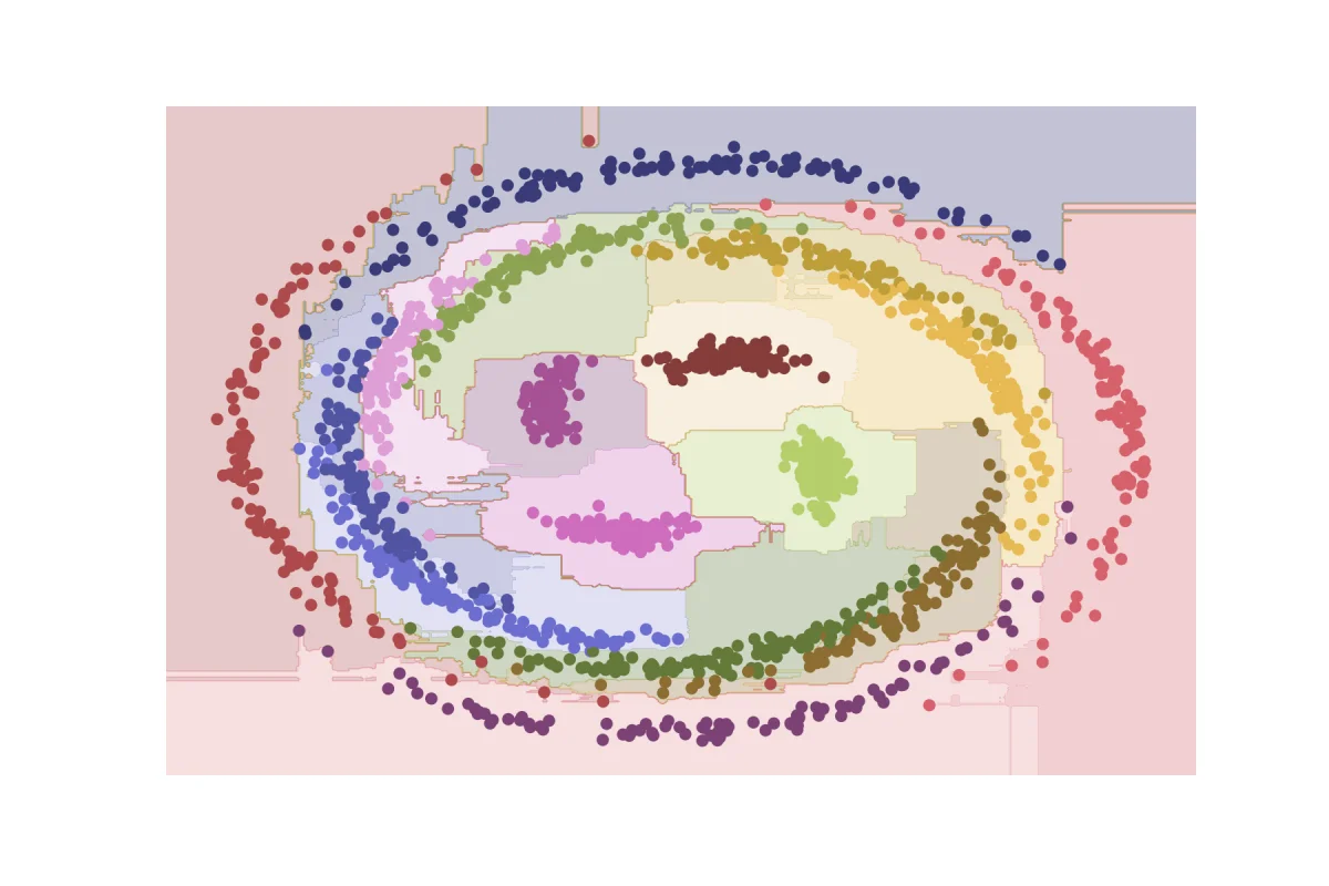 (full size, opens in a new tab)
05 The simulation
A single-channel 16-QAM link at 128 Gbit/s, simulated in VPI: a transmitter with adjustable launch power, a loop of 80 km dispersion-shifted fibre spans with low-noise amplifiers, and a coherent receiver. The loop runs up to 64 times, 5120 km. Amplifier noise is kept small so the nonlinear effects dominate. A link counts as reliable while its symbol error rate stays below 10⁻⁵.
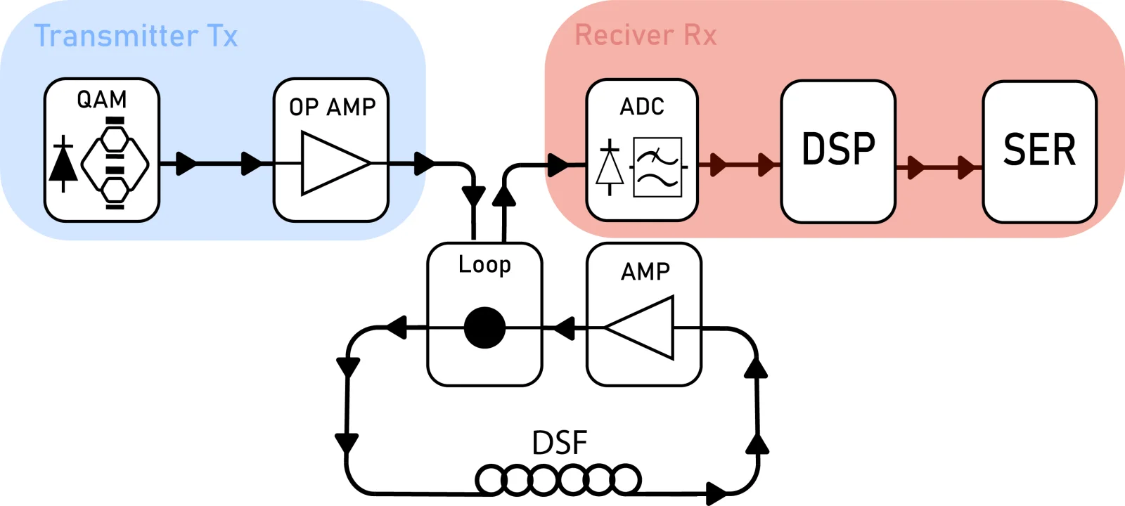
 (full size, opens in a new tab)
 (full size, opens in a new tab)
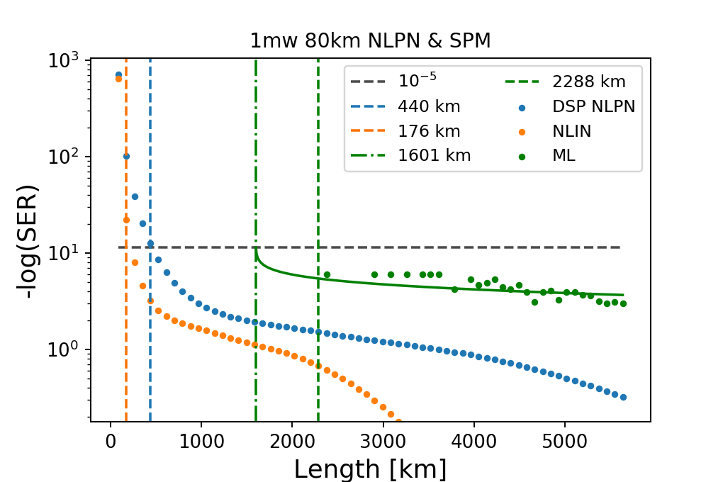
Each launch power gives three error curves against distance: the raw signal, a compensation scheme derived from the physics of the link, and the learned receiver. The vertical lines mark where each one stops being reliable.
Y: symbol error rate · X: distance, km● Raw■ Compensated┆ Reach
- Reach, raw
- 160 km
- Reach, comp.
- 400 km
- Ratio
- 2.5×
Show the numbers
| Power | Compensated reach | Raw reach | Ratio |
|---|---|---|---|
| 0.17 mW | 1600 km | 1040 km | 1.5× |
| 0.25 mW | 1360 km | 720 km | 1.9× |
| 0.5 mW | 800 km | 400 km | 2.0× |
| 1 mW | 400 km | 160 km | 2.5× |
| 1.5 mW | 560 km | 400 km | 1.4× |
| 2 mW | 560 km | 400 km | 1.4× |
06 Key figures
| Parameter | Value | Unit |
|---|---|---|
| Format, single channel | 16-QAM, 128 | Gbit/s |
| Fibre span | 80 | km |
| Longest link simulated, 64 spans | 5120 | km |
| Reliable link | SER < 10⁻⁵ | |
| Launch power, learned-receiver comparison (thesis) | 1 | mW |
| Reach gain, learned receiver, simulated | 2.5 simulated; up to 9.4 by exponential fit | × |
| WDM test system, 5 wavelengths × 2 polarisations (10 channels) | 1280 | Gbit/s |
| Channel spacing, WDM | 50 | GHz |
07 Result
On the long single-channel link, the learned receiver matches the compensation scheme that knows the link, with no information about the link at all, and stretches reach 2.5 times. An exponential fit to its error rate suggests up to 9.4 times; the simulation ran 4096 symbols per frame, too few to count rarer errors directly. On the ten-channel WDM system no clear gain shows: noise from neighbouring channels changes in time, and a fixed decision map cannot follow it.
The conclusion: on a long-haul link, knowledge of the system can be replaced by learning.
08 Where it leads now
The idea I still like from this thesis: you do not have to model the Kerr effect, or know every property of the fibre, to undo what it does. Send a known pattern first, let the receiver learn the distortion, and each span calibrates itself quickly. The same idea, learning the distortion instead of modelling it, took me into radio, where I worked on digital pre-distortion for power amplifiers.